on
Final 2022 Election Prediction
This blog is part of a series for Gov 1347: Election Analytics, a course at Harvard University taught by Professor Ryan D. Enos.
Introduction
It’s finally here.
Election Day has finally arrived, and I know my lovely blog audience has been eagerly awaiting my final prediction for the “most important election in our lifetime” (or as every election ever seems to be). This post will provide a full breakdown of my final national model - which predicts both Democrats’ national two-party vote share and the number of Democratic House seats - and an interpretation of the results.
Formula and Variables
Since two weeks ago, I made several changes to the variables I incorporate into my model. Notably, I have decided to leave out data from the 2020 election entirely due to the highly unusual circumstances of the election taking place during the COVID-19 pandemic.


Above are the formulas for the vote share and seat share versions of the model. As you can see, both use the same independent variables, differing only in the dependent variable. Below I break down each of the four independent variables I’ve chosen to use for my model:
1. Unemployment rate: Specifically, I use the percent change in the unemployment rate between the third and fourth quarter of the election year. I use the last few months of unemployment data since it is what people will be experiencing at the time of the election, and I now am using percent change to better capture major changes to unemployment close to an election that would be more noticeable to voters.
2. Real disposable income: I decided to include another economic variable, seeing as how often the economy is played up as one of the most important issues in this election and almost every other election. Similarly to the unemployment rate variable, I use the percent change in RDI between the third and fourth quarter of the election year.
3. Average democratic generic ballot support: Based on past elections, the generic ballot continues to be a powerful tool for helping us predict the final results of the election. I incorporate the last 100 days of generic ballot polls before the election since the closer the election is, the closer the polls seem to converge on the final result.
4. Incumbent party of the president: I decided to just focus on this incumbency variable, based on the conventional wisdom that midterm elections are bad for the incumbent president’s party specifically, even if the opposing party is in control of the House or Senate. It measures whether the incumbent president at the time of the election is a Democrat (1) or a Republican (0).
Regression Tables
Out-Of-Sample Testing
For both the vote share and seat share regressions, I will pull out the data from 2018 and use it to test the model’s ability to predict values outside of the sample.
##         1
## -1.079743
When taking the data for the year 2018 out of the original model and predicting it as if it were outside the sample, the predicted Democratic vote share is about 1.08% less than the true result for 2018. Although 1.08 isn’t a huge difference, in terms of the popular vote for the House, it can mean the difference between winning or losing the majority, so this test shows that there is still quite a bit of uncertainty using this model to predict elections outside of the sample.
##        1
## 14.25989
The model’s uncertainty is even more visible when looking at seat share. Here, the model’s prediction is about 14 seats higher than the actual result for 2018. Again, 14 seats is not huge, but it can definitely sway the majority one way or the other.
Final Prediction
Below represents what you’ve all been waiting for: how will the Democrats fare on Tuesday??
##        fit      lwr      upr
## 1 49.70226 45.48201 53.92251
My model predicts that Democrats will win about 49.7% of the popular vote. This margin would represent an extremely close race, though with a slight edge for the Republicans. The model suggests we could see a vote share for Democrats anywhere between 45.48% and 53.92%, a range that’s somewhat wide, reflecting the uncertainty of the model and of this election in general.
##        fit      lwr     upr
## 1 214.7462 171.9684 257.524
As for seats, my model predicts that Democrats will win about 215 seats. This result means that Democrats are projected to lose their majority in the House by just three seats, the slimmest of margins. The model suggests we could see a seat share for Democrats anywhere between 172 seats and 258 seats, a very wide range. This suggests to me that the seat share model is even more uncertain of what to predict for the final number of seats that Democrats will win, since it includes both a Republican landslide and Democratic landslide scenario.
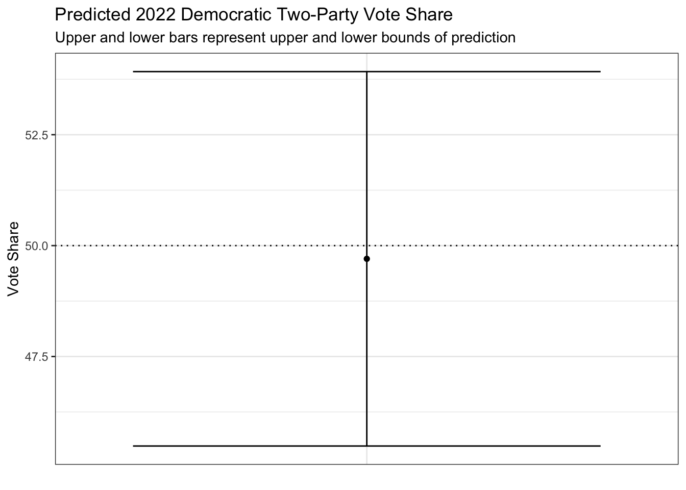
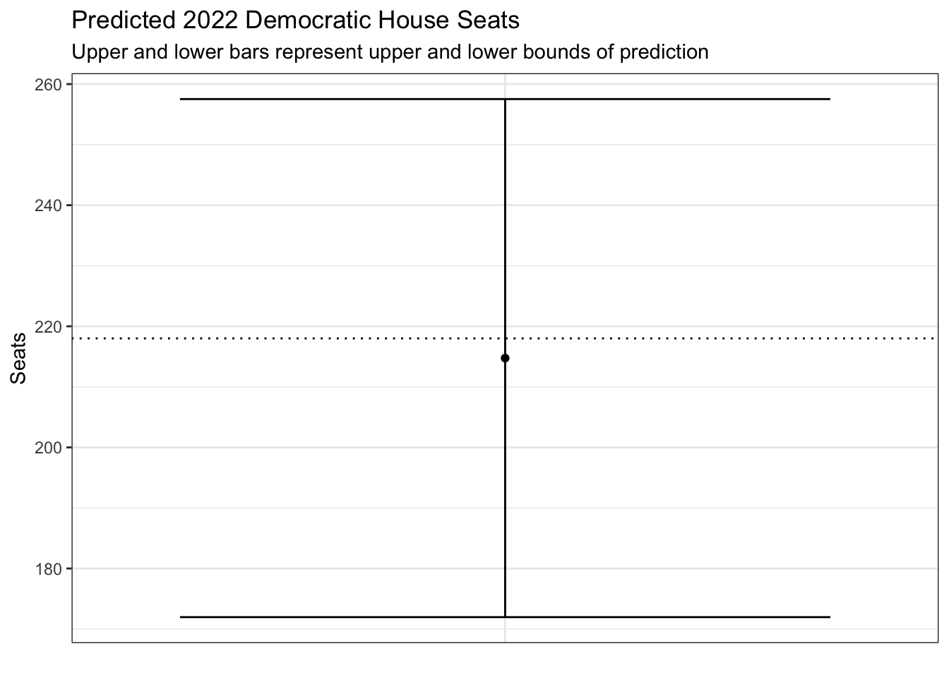
Finally, above are visualizations of my prediction intervals. As you can see, Democrats are just shy of a majority of the popular vote and seats, but the upper and lower bounds are so large that technically anything is possible.