on
Blog Post 6 - The Ground Game
This blog is part of a series for Gov 1347: Election Analytics, a course at Harvard University taught by Professor Ryan D. Enos.
Introduction
Last week, we looked at the “air war,” where political campaigns fight each other through political advertisements that promote each side and/or attack the other side. Now, we are about to take the war to the ground as we look at how campaigns try to influence voter turnout in their favor.
“Turnout” isn’t just about the number or percentage of voters showing up to the polls - it’s about who shows up and why. Campaigns usually invest in on-the-ground operations to do two things:
1. Mobilize voters: For a candidate, having voters agree with you is not enough - they need to show up! By getting supporters to stop procrastinating filling out their mail-in ballot or helping them get to the polls on election day, campaigns can tap into their base and increase the number of votes they receive. Ideally, a candidate would want more people from their side to show up than the other side!
2. Persuade voters: Besides getting people who already support or lean towards a candidate to actually go vote, campaigns also try to convince people who are on the fence or do not have strong leanings either way to join their side and vote.
What Can Predict Turnout?
In this post, I wanted to look at two different variables - expert predictions and spending on political ads - and see if they had any sort of relationship to turnout.
For expert predictions, I used data provided from class a few weeks ago that provides average expert ratings for many House districts. For many other districts, there are no ratings, but presumably that is because these districts were solidly in the camp of one party, and experts would likely want to focus on the races that are more competitive. Nevertheless, I included as much data as was available from 2012 to 2020.
For ad spend, I used last week’s data, but instead of limiting the data to just the few months before an election, I included all ad spend data available, as some districts did not have ad spend data for the few months before an election.
Expert Predictions Turnout Model
| Characteristic | Beta | 95% CI1 | p-value |
|---|---|---|---|
| (Intercept) | 0.59 | 0.56, 0.62 | <0.001 |
| avg_rating | -0.01 | -0.01, 0.00 | 0.005 |
| 1 CI = Confidence Interval | |||
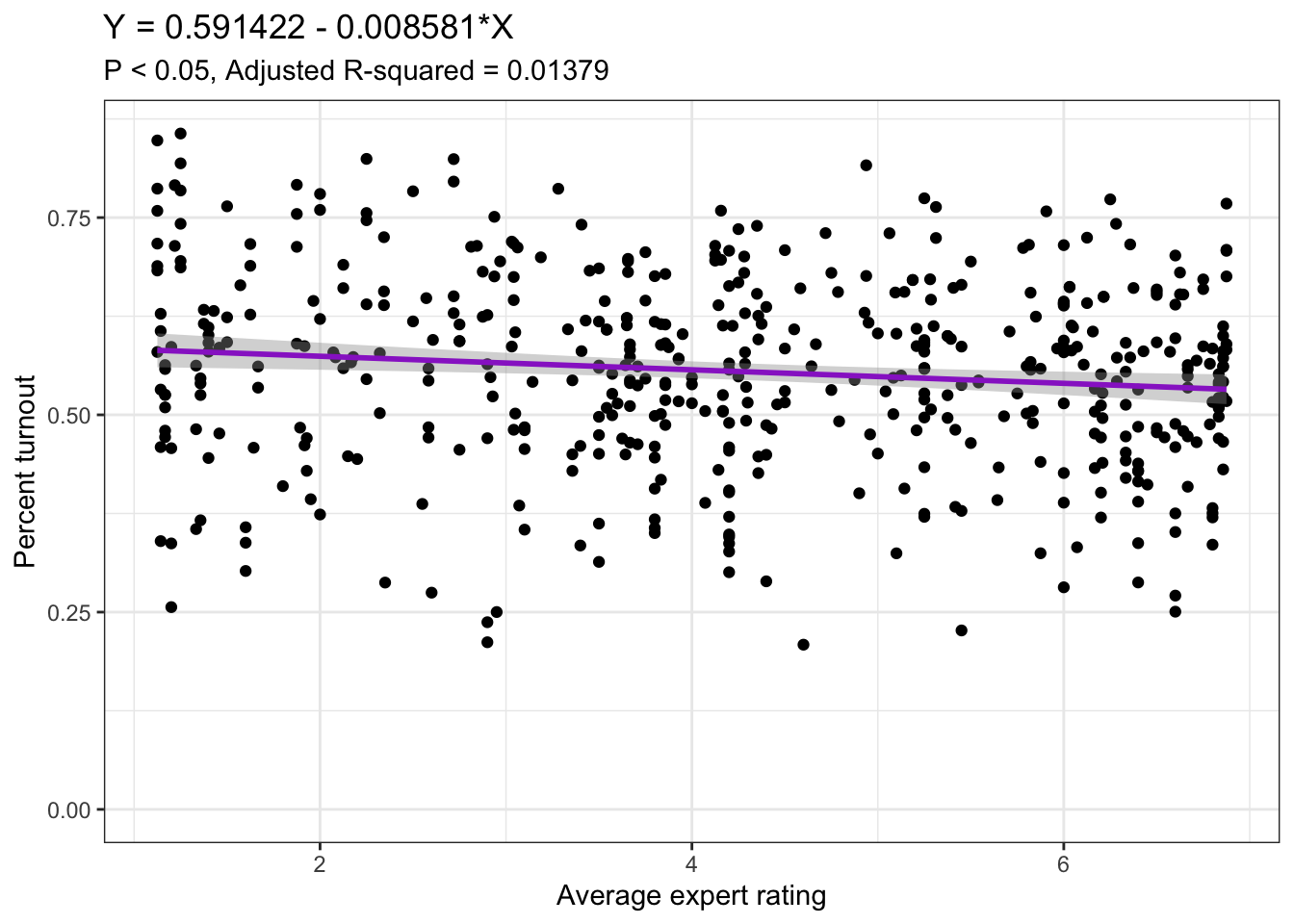
The avg_rating variable is coded on a scale from 1 to 7, with 1 representing an average expert rating of “Solid Democratic” for a district and 7 representing an average expert rating of “Solid Republican” for a district. The table and plot above suggest that an increase of 1 in rating - a one-unit shift towards Republicans - has just the slightest negative effect on percent turnout in an election. The coefficient is statistically significant, but the adjusted R-squared is only 0.01379, which suggests that this model is not too great at telling us how much average expert ratings can really be predictive of turnout, and since the effect is so small either way, it also doesn’t tell us much about how much ground campaigns do anything for turnout.
Ad Spend Turnout Model
| Characteristic | Beta | 95% CI1 | p-value |
|---|---|---|---|
| (Intercept) | 0.48 | 0.47, 0.49 | <0.001 |
| total_cost | 0.00 | 0.00, 0.00 | <0.001 |
| 1 CI = Confidence Interval | |||
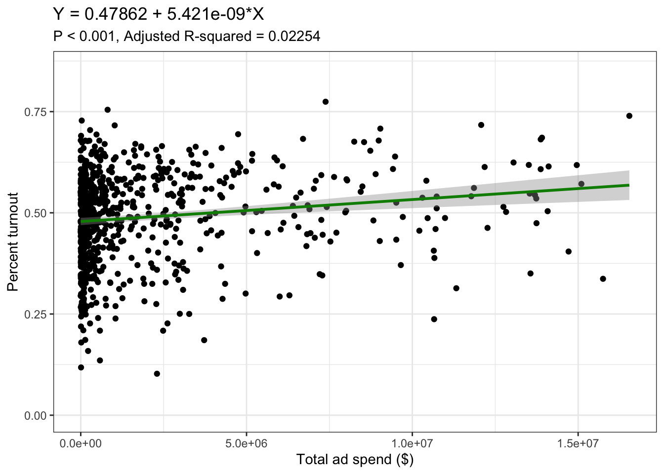
On the other hand, ad spend seems to have a different relationship to turnout based on this model. The more that each party spent on ads, the higher turnout seems to go based on the plot. However, most of the points are clustered to the left, so we have more limited data for those much bigger ad spends. In addition, although the adjusted R-squared of 0.02254 is higher than the expert prediction model, it is still very very low, so this model in particular would not be ideal for making predictions. If this model were much more robust and came to a similar conclusion, one could argue that what happens during the air war of political ads drives at least some people to go vote and potentially convinces others to pick a side, especially when tons of money is poured in.
Updated 2022 Model for CA-27
Like last week, I could not get district-level predictions to work on the aggregate level, but I was able to build a model incorporating turnout, incumbency, and expert predictions to update my forecast for CA-27, the district I am following.
##
## Call:
## lm(formula = DemVotesMajorPercent ~ avg_rating + incumb + turnout,
##     data = model_data)
##
## Residuals:
##      Min       1Q   Median       3Q      Max
## -13.5164  -1.9577  -0.0109   1.8549  18.3589
##
## Coefficients:
##             Estimate Std. Error t value Pr(>|t|)
## (Intercept) 62.33900    0.80722  77.227   <2e-16 ***
## avg_rating  -2.90114    0.08318 -34.877   <2e-16 ***
## incumbTRUE  -0.38410    0.30317  -1.267    0.206
## turnout     -1.81989    1.21986  -1.492    0.136
## ---
## Signif. codes:  0 '***' 0.001 '**' 0.01 '*' 0.05 '.' 0.1 ' ' 1
##
## Residual standard error: 3.247 on 497 degrees of freedom
##   (15566 observations deleted due to missingness)
## Multiple R-squared:  0.7174, Adjusted R-squared:  0.7157
## F-statistic: 420.5 on 3 and 497 DF,  p-value: < 2.2e-16
This model has an adjusted R-squared of 0.7157, which is impressively high. However, only the avg_rating variable is statistically significant, which is not too surprising since better expert ratings for Republicans will likely translate to lower Democratic vote percentages.
##        fit      lwr      upr
## 1 49.47535 43.08016 55.87054
Above is the predicted Democratic percent voteshare for the district based on this model. Last week, both the models I used suggests Democratic challenger Christy Smith would win just slightly over 50% of the vote, but this model predicts she will win about 49.48% of the vote, which would be an extremely narrow loss. The lower and upper bounds are wide, but unlike last week, they are arguably more realistic possibilities. Nonetheless, I continue to expect this election to be a nail-biter.