on
Blog Post 4 - Incumbency and Expert Predictions
This blog is part of a series for Gov 1347: Election Analytics, a course at Harvard University taught by Professor Ryan D. Enos.
Introduction
As we discussed last week, the FiveThirtyEight and the Economist each run their own election forecasts, with each of them having similarities and differences in their methodology when it comes to how to incorporate variables like polling and the fundamentals. One interesting difference, however, between the two models especially caught my attention - FiveThirtyEight’s model (specifically the Deluxe version) includes other forecasters’ ratings of the different races. Although adding their ratings to a model could feel like “cheating,” they could be considered as another one of several indicators of how each party is doing, similar to other variables like polling or the economy.
Are the Experts Really Experts? A Look at 2018
Elections can be weird, and 2018 was no exception. The first midterm of Donald Trump’s presidency, the election ended up giving both parties a result to be happy about, as each chamber of Congress moved in opposite directions, with Democrats winning a net of 41 seats and taking the House majority at the same time that Republicans won a net of 2 seats and held on to control of the Senate. This outcome seems strange considering midterms are usually unfavorable all around for the party in power. In fact, the last time that the incumbent president’s party made net gains in one chamber and suffered net losses in the other chamber was in 1970!
Elections like these make it that much more interesting to follow the predictions of the experts. To analyze their accuracy in 2018, I used a dataset provided by Ethan Jasny - another student in this course - which contains expert race ratings of all 435 congressional districts by the three expert organizations that FiveThirtyEight uses. Using this data and shapefile data from previous weeks, I was able to visualize the actual two-party voteshare for each district in 2018 and the average expert race ratings for all of the districts.
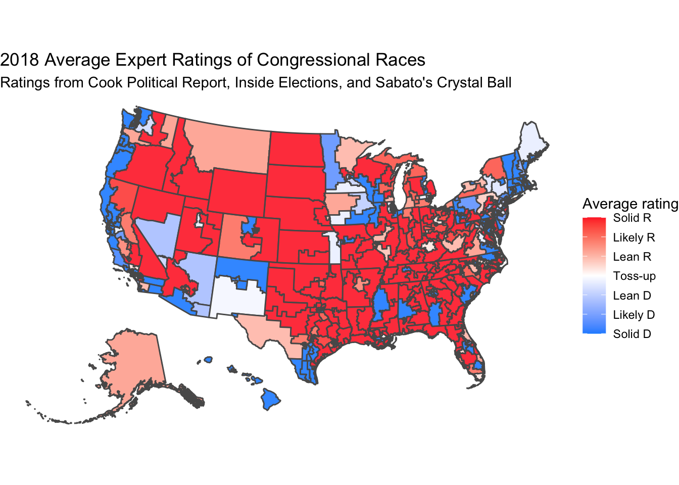
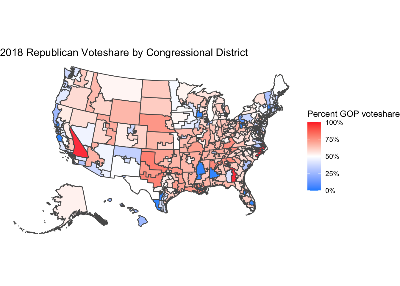
The top graph shows the average expert ratings, while the bottom graph shows the final Republican voteshare. Despite the more intense colors on the expert ratings graph, which I believe is due to more of a concentration of datapoints on the extremes than for the actual voteshares, the experts can generally predict the results in most districts, including in more competitive areas.
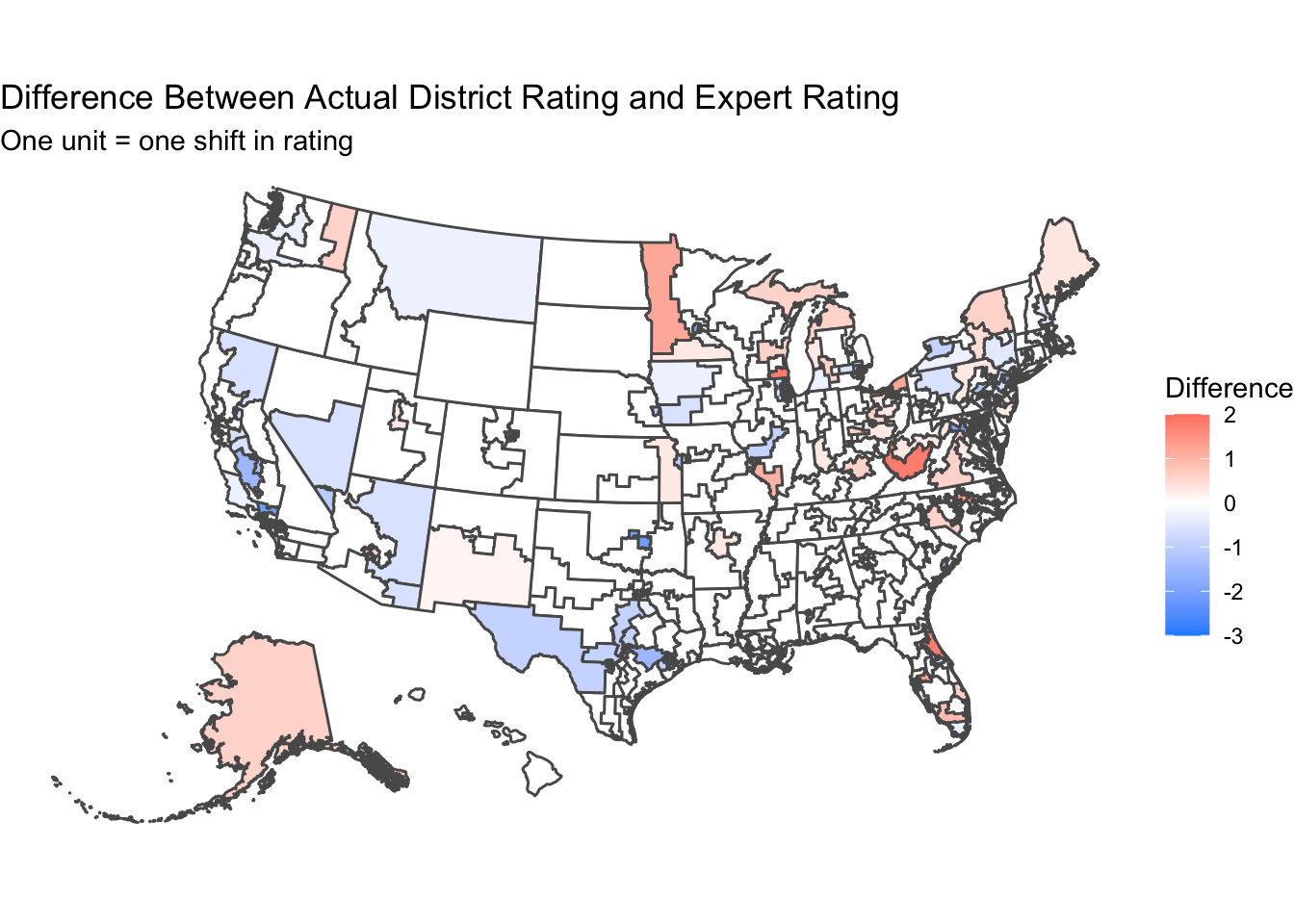
For an easier to see comparison, I made a third map which shows the difference in the actual result from the average expert prediction for a given district. I grouped the different voteshares into the same categories as the expert predictions based on how large Republicans won or lost in their districts. On this graph, positive numbers mean Republicans did better than the expert prediction, while negative numbers mean Republicans did worse. Throughout most of the country, the difference is close to 0, but that can likely be attributed to the fact that most races in the House are not competitive. Instead, you can see a pattern of underestimating Democrats in some areas like California, Arizona, and Texas while underestimating Republicans in New York, Florida, and the Rust Belt. However, many of these districts seemed to have only shifted one category, which may not have always led to the seat flipping outright. Overall though, the experts to rarely be wrong by much, if at all, even in elections like 2018.
Updating my Model
Based on this analysis, I wanted to try and add expert ratings to my current model, though with how the data was structured, using it for my model that still uses national-level data for incumbent party voteshare would be tougher. The method I tried was to essentially take the expert district ratings from 2010 to 2020 and take the average, by year, across the whole country. I added this as another independent variable alongside the fundamentals and polling and ran a linear regression, the results of which are below.
##
## Call:
## lm(formula = H_incumbent_party_majorvote_pct ~ avg_pct_chg +
##     UNRATE + avg_support + avg_expert, data = dat_poll_fun_exp)
##
## Residuals:
##     Min      1Q  Median      3Q     Max
## -0.8714 -0.6582 -0.2920  0.6910  1.7921
##
## Coefficients:
##               Estimate Std. Error t value Pr(>|t|)
## (Intercept) -128.82710    3.52172  -36.58   <2e-16 ***
## avg_pct_chg  -14.65479    0.39621  -36.99   <2e-16 ***
## UNRATE         1.12717    0.03301   34.15   <2e-16 ***
## avg_support    2.33130    0.04172   55.88   <2e-16 ***
## avg_expert    17.27443    0.42114   41.02   <2e-16 ***
## ---
## Signif. codes:  0 '***' 0.001 '**' 0.01 '*' 0.05 '.' 0.1 ' ' 1
##
## Residual standard error: 0.7884 on 762 degrees of freedom
##   (1343 observations deleted due to missingness)
## Multiple R-squared:  0.8517, Adjusted R-squared:  0.8509
## F-statistic:  1094 on 4 and 762 DF,  p-value: < 2.2e-16
Interestingly, the coefficients are all statistically significant, and the adjusted R-squared since adding the “avg_expert” variable skyrocketed to 0.8509. However, I have my doubts about the true validity of this model, as the sample size for expert ratings is very small, and the method that I used condenses all ratings from across the country, which may not produce the most accurate results.
##        fit      lwr    upr
## 1 32.32693 30.67887 33.975
The model gave me an incredibly strange prediction - a 32.33% voteshare for the incumbent party! While not impossible, this result would be incredibly unlikely! As suspected, including expert predictions in this way caused my model to perform much worse than before, which means next week, I will reevaluate which other variables I should consider instead.