Introduction

This week, we took a look at the role that polling plays in election forecasting. Polls of all kinds are conducted weeks, months, or even years before an election, but as we can see in this graph of FiveThirtyEight’s aggregation of generic ballot polls for the 2022 midterms, polls are much more frequently conducted as election day gets closer.

As Gelman and King (1993) argue, the preferences of voters reported in polls throughout the campaign are not “informed” nor “rational,” with voters instead making a decision on who to vote for based on their “enlightened preferences” formed throughout the campaign and other cues like ideology and party identification. Thus, when updating last week’s models that only incorporated economic variables - CPI and unemployment - it will be interesting to see whether fundamentals alone or polls combined with fundamentals will be more predictive of this election.

What Do Forecasters Do?

Before I begin tinkering with my model, I want to compare and contrast two well-known election forecasters and their approaches to modeling the election.

FiveThirtyEight’s model, created by Nate Silver, has a very detailed methodology page. In summary, their model takes in as many local polls as possible, making different kinds of adjustments to them and incorporating the fundamentals to produce forecasts for each race after thousands of simulations. Their model is split into three versions: a “lite” model that only incorporates adjusted district-by-district polls and CANTOR (a system that infers polls in districts with little to no actual polling); a “classic” model that combines the lite model with fundamentals, non-polling factors like fundraising and past election results; and a “deluxe” model that combines the classic model with the race ratings by “experts”, namely the Cook Political Report, Inside Elections, and Sabato’s Crystall Ball. FiveThirtyEight uses an algorithm to weigh polls based on their sample size, their recency, and the pollster rating, with an emphasis on having a diversity of polls. They do note that their House model, unlike their Senate and governor models, is less polling-centric since polling for House races is more sporadic and potentially unreliable, making fundamentals a more significant factor where House polling is sparse.

The Economist’s model seems to weigh polling somwehat more, though it still most definitely takes fundamentals and other factors into account. The model first tries to predict a range of outcomes for the national House popular vote, using generic ballot polls (which FiveThirtyEight use more as adjustments for local polls), presidential approval ratings, the average results of special elections held to fill vacant legislative seats, and the number of days left until the election. The model then tries to measure each district’s partisan lean, incorporating more fundamentals and interestingly, an adjustment for political polarization. Finally, the model incorporates local polling, adjusting polls as needed, and simulates the election tens of thousands of times, coming up with a final prediction.

Which model do I prefer? In my opinion, both models are very well-thought out, but I prefer FiveThirtyEight’s model somewhat more. I like that their model is set up into three versions, which help give readers an idea of the individual impact of polls and fundamentals as well as the wisdom of respected expert forecasters. I also prefer how their model is probabilistic, which means they are not forgetting about all the uncertainty that comes with these elections!

Updating My Model

Last week, my models based on economic variables did not perform too well. For the comparison against polling, one change I would like to make is combining CPI and unemployment into one “economic fundamentals” model that will ideally perform better than each variable individually. Last week, I also experimented with leaving out presidential election years, but for this post, I will be considering all election years.

## 
## Call:
## lm(formula = H_incumbent_party_majorvote_pct ~ avg_pct_chg + 
##     UNRATE, data = dat_fun)
## 
## Residuals:
##     Min      1Q  Median      3Q     Max 
## -6.9172 -0.9947  0.3410  2.0728  6.7196 
## 
## Coefficients:
##             Estimate Std. Error t value Pr(>|t|)    
## (Intercept)  46.6965     1.9310  24.183   <2e-16 ***
## avg_pct_chg   1.0069     0.5606   1.796   0.0813 .  
## UNRATE        0.6766     0.3180   2.128   0.0407 *  
## ---
## Signif. codes:  0 '***' 0.001 '**' 0.01 '*' 0.05 '.' 0.1 ' ' 1
## 
## Residual standard error: 3.083 on 34 degrees of freedom
## Multiple R-squared:  0.2061, Adjusted R-squared:  0.1594 
## F-statistic: 4.412 on 2 and 34 DF,  p-value: 0.01979

Above is a quick summary of my new fundamentals-only model. In this model, the unemployment rate one month before the election (but not the average percent change in CPI in the last 3 months before the election) appears to have a statistically significant positive effect on the house incumbent party voteshare.

## [1] 2.955645

In terms of in-sample fit, the above number represents the mean squared error, which on its own does not mean much, but we will use it to this model to the other models. The adjusted R-squared is 0.1594, which is better than most of my models from last week, but it is still relatively low.

## 
## Call:
## lm(formula = H_incumbent_party_majorvote_pct ~ avg_pct_chg + 
##     UNRATE + avg_support, data = dat_poll_fun)
## 
## Residuals:
##     Min      1Q  Median      3Q     Max 
## -7.2833 -2.8399  0.0531  1.9505  8.0226 
## 
## Coefficients:
##             Estimate Std. Error t value Pr(>|t|)    
## (Intercept) 40.62411    0.81469   49.87  < 2e-16 ***
## avg_pct_chg  2.48015    0.09932   24.97  < 2e-16 ***
## UNRATE       0.48912    0.03496   13.99  < 2e-16 ***
## avg_support  0.08637    0.01671    5.17 2.57e-07 ***
## ---
## Signif. codes:  0 '***' 0.001 '**' 0.01 '*' 0.05 '.' 0.1 ' ' 1
## 
## Residual standard error: 2.792 on 2106 degrees of freedom
## Multiple R-squared:  0.2872, Adjusted R-squared:  0.2862 
## F-statistic: 282.9 on 3 and 2106 DF,  p-value: < 2.2e-16

Above is a quick summary of the combined polls and fundamentals model. All of the variables are statistically significant!

## Warning in lm_poll_fun$model$H_incumbent_party_majorvote_pct -
## lm_fun$fitted.values: longer object length is not a multiple of shorter object
## length

## [1] 4.344127

The mean squared error is higher for this model, but based on the warning message, this may not be an accurate measure of in-sample fit. The adjusted R-squared for this model is 0.2833, which is significantly higher than the other model’s value of 0.1594, making this model have a better in-sample fit.

Comparing Models

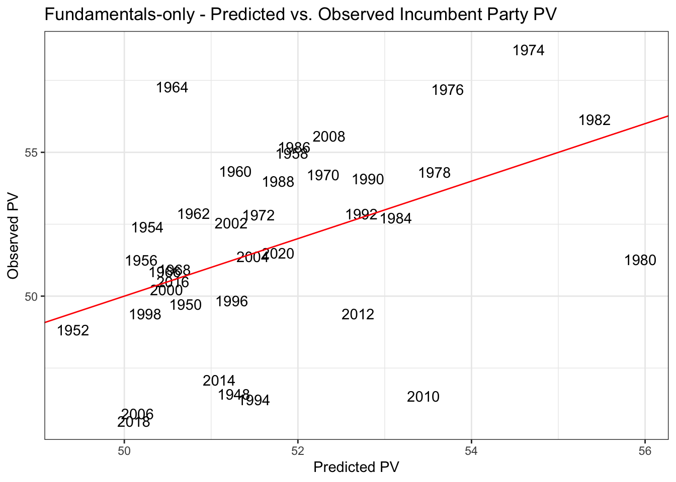
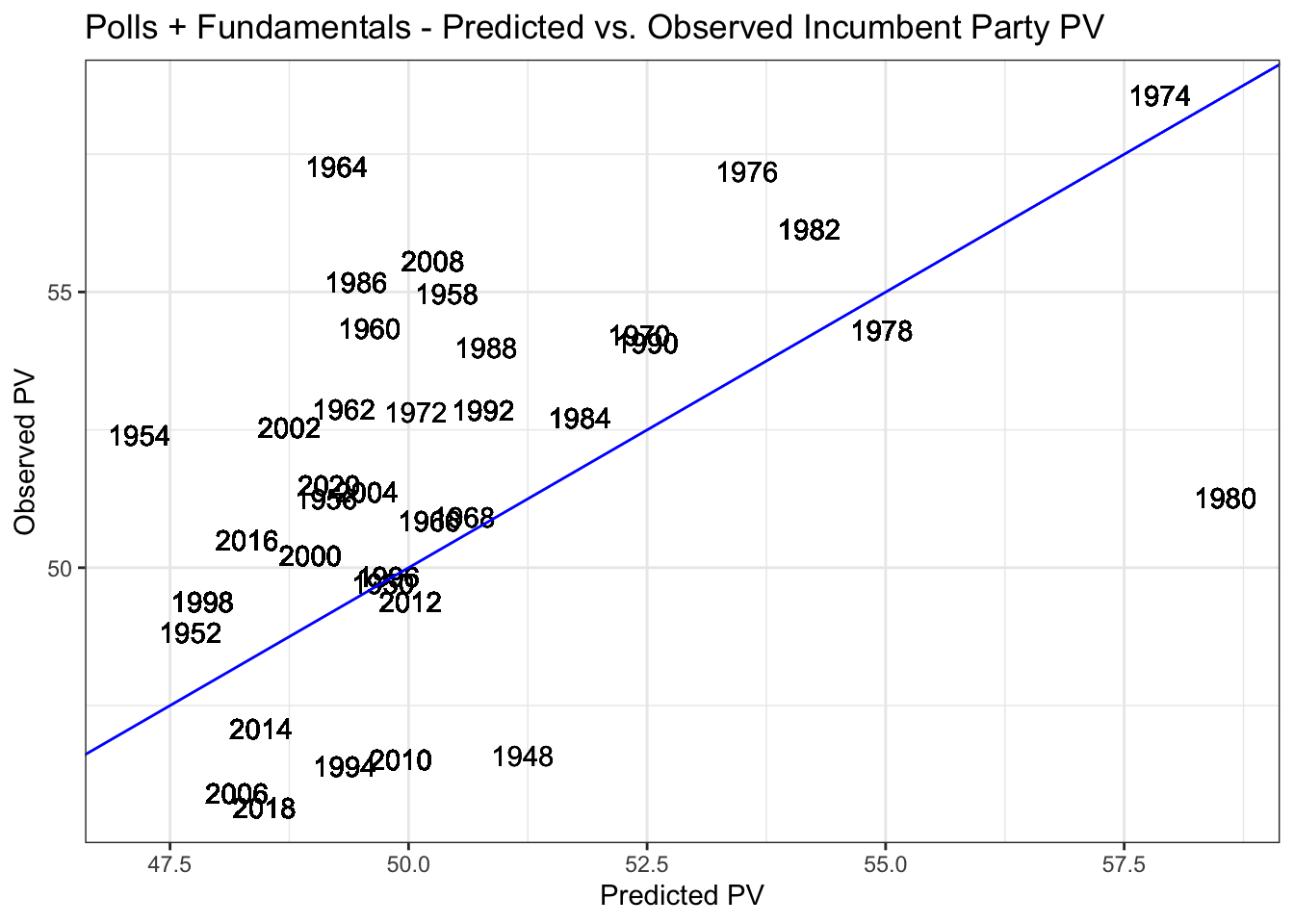
The above are predicted vs. observed incumbent party voteshares for each of my models. Although neither are necessarily good fits for the data, both models, particularly the polls + fundamentals models, are an improvement over last week’s models!

2022 Predictions

Fundamentals-only

##        fit      lwr      upr
## 1 50.01443 43.51534 56.51353

Polls + Fundamentals

##        fit      lwr      upr
## 1 48.24779 42.76806 53.72752

Above are the predictions each model has made for the incumbent party voteshare for the 2022 midterms. The fundamentals-only model predicts Democrats will win about 50.01% of the vote, while the polls + fundamentals model suggests Democrats will fall short of winning the majority of the popular vote with about 48.25% of the vote. The latter model presents the most pessimistic outcome for Democrats out of all of my models so far. Next week, I am interested to see if and how this will change.

References

Gelman, A., & King, G. (1993). Why Are American Presidential Election Campaign Polls So Variable When Votes Are So Predictable? British Journal of Political Science, 23(4), 409-451. doi:10.1017/S0007123400006682